DJH Energy Consulting
Dan J. Hartmann
P.O. Box 271
Fredericksburg, Texas 78624
210-508-7455
djhec@ktc.com.
Dan J. Hartmann
P.O. Box 271
Fredericksburg, Texas 78624
210-508-7455
djhec@ktc.com.
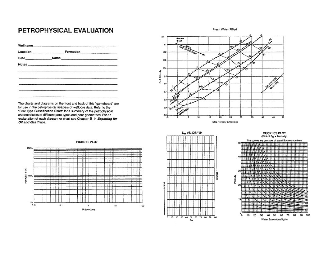
PETROPHYSICAL EVALUATION GAME BOARD
Question: How to process log analysis data to derive porosity, lithology, fluid type and water saturation with minimal error bars.
Protocol:
A. Assimilate the data.
1. Gather the SP, GR, resistivity, density, neutron, sonic, MWD, LWD, mud log, NMR and any cased hole logs available.
2. Display them all together at common depth and evaluate integrated cure response, shape and scales.
3. Define mappable containers (sequence stratigraphic cycles) and subdivide into flow units (intervals of uniform porosity,
resistivity and gamma ray).
4. Identify each flow unit with a unique number, numbering from top (1) to base (i.e. 15).
5. Integrate these flow units with appropriate intervals from the Pore Geometry Game Board.
B. Plot the data.
1. Plot density and neutron log values.
a. Raw data (bulk density and neutron limestone porosity) move neutron up and density right to intercept.
b. Computed porosity (i.e. using limestone matrix).
1. Post neutron value on LS Matrix line.
2. Post density value on LS line and move neutron vertically and density horizontally until they intercept.
c. Point at intercept reflects lithology, clay content and fluid type (gas or liquid).
d. Correct porosity for clay shift and gas shift.
e. Identify each point by flow unit numbers, draw ellipses around populations and relate to core data populations.
2. Plot D/N porosity (y-axis) from step 1 to resistivity (x-axis) (corrected for infusion and thin bed effects) on Pickett Plot.
a. Add flow unit numbers and violate populations.
b. Post Rw at 100% porosity and draw the 100% Sw line using the proper cementation exponent ("M").
1. "M" = 2 for clean sandstone and intercrystalline carbonate or intergranular carbonate.
2. "M" = 1.7 for clay cemented sandstone.
3. "M" = 2.5 +/- for vuggy/oomoldic carbonates.
c. Add an Sw grid (Sw = 70,50, 25, 10%) by computing an Rt for each value of Sw, using Rt = Ro/Sw n (where "n" = 2)
at constant porosity.
1. Set Ro = 1 by definition.
2. At Ro = 1, draw a constant porosity at 100% Sw.
3. Post the Rt values (2 = 70%, 4 = 50%, 16 = 25%, 100 = 10%) on the porosity line, and draw lines parallel to
100% Sw through each of these points. This creates a template for estimating a quick look Sw for each flow unit.
3. Plot Sw by flow unit to depth to form an Sw profile. Since Sw is a function of height in the reservoir and pore type, this
profile can be integrated with a curve derived by dividing core perm by fractional core porosity and plotting it on
the same depth chart. The two curves integrate port size with Sw, at a specific elevation in the hydrocarbon
column.